German Economic Analysis using the Destatis Genesis Database in R

# Pakete laden
library(ggplot2)
library(dplyr)
library(restatis)
library(data.table)

# API 
#gen_auth_save("genesis", use_token = TRUE) 

colors <-  c("Nominal" = "#7570B3", "Real" = "#D95F02", "Accent" = "#1B9E77", "CPI" = "#B0E0E6")

theme_set <- function() {
  ggplot2::theme_minimal(base_size = 12) + 
  ggplot2::theme(
    panel.grid.major = element_blank(),
    panel.grid.minor = element_blank(),
    axis.line = element_line(colour = "grey50"),
    plot.title = element_text(face = "bold", size = 16, hjust = 0),
    plot.subtitle = element_text(size = 12, hjust = 0),
    legend.position = "bottom",
    legend.title = element_blank(), 
    plot.background = element_rect(fill = "white", color = NA)
  )
}

bip_raw <- gen_table("81000-0001", database = "genesis",  silent = TRUE)
cpi_raw <- gen_table("61111-0001", database = "genesis")

GDP Analysis

GDP Development

bip_nominal <- bip_raw |>
  filter(value_variable_code == "VGR014",
         value_unit == "unit app.",
         `2_variable_attribute_label` == "At current prices (bn EUR)") |>
  mutate(time = as.integer(time),
         value = as.numeric(value)) |>
  select(time, value) |>
  rename(nominal = value) |>
  setDT()

bip_real <- bip_raw |>
  filter(value_variable_code == "VGR014",
         value_unit == "unit app.",
         `2_variable_attribute_label` == "Price-adjusted, chain-linked volume data (bn EUR)") |>
  mutate(time = as.integer(time),
         value = as.numeric(value)) |>
  select(time, value) |>
  rename(real = value)|>
  setDT()

bip_combined <- full_join(bip_nominal, bip_real, by = "time") %>% 
  filter(time >= 1992) 

cpi_rate <- cpi_raw |>
  filter(value_unit == "%") |>
  mutate(
    time = as.integer(time),
    cpi_rate = as.numeric(value)
  ) |>
  filter(time >= 1992) |>
  select(time, cpi_rate)|>
  setDT()

bip_cpi <- merge(bip_combined, cpi_rate, by = "time", all.x = TRUE)

## get max and factor values
gdp_max <- max(bip_cpi$nominal, na.rm = TRUE)
cpi_max <- max(bip_cpi$cpi_rate, na.rm = TRUE)
scale_factor <- gdp_max / cpi_max

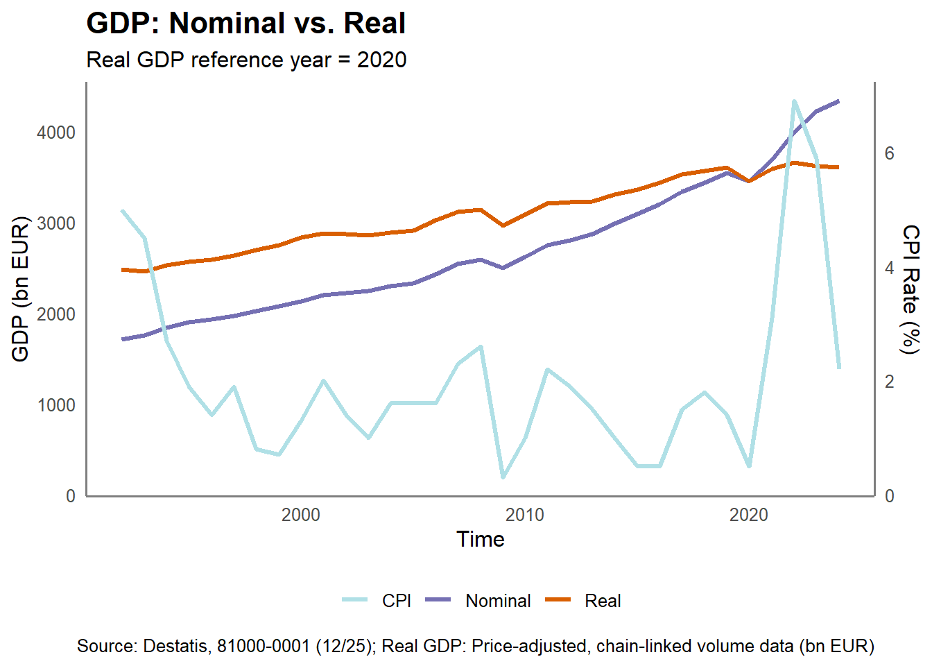
ggplot(bip_cpi, aes(x = time)) +
  geom_line(aes(y = nominal, color = "Nominal"), linewidth = 1.2) +
  geom_line(aes(y = real, color = "Real"), linewidth = 1.2) +
  geom_line(aes(y = cpi_rate * scale_factor, color = "CPI"), linewidth = 1.2) +
  labs(
    title = "GDP: Nominal vs. Real",
    subtitle = "Real GDP reference year = 2020",
    x = "Time",
    y = "GDP (bn EUR)",
    caption = "Source: Destatis, 81000-0001 (12/25); Real GDP: Price-adjusted, chain-linked volume data (bn EUR)"
  ) +
  scale_color_manual(values = colors) +
  theme_set() +
  scale_y_continuous(
    name = "GDP (bn EUR)",
    sec.axis = sec_axis(transform = ~ . / scale_factor, name = "CPI Rate (%)")
  ) 

BIP Growth Rate

bip_growth <- bip_combined |>
  arrange(time) |>
  mutate(nominal_growth = (nominal / lag(nominal) - 1) * 100,
         real_growth = (real / lag(real) - 1) * 100)

ggplot(bip_growth, aes(x = time)) +
  geom_line(aes(y = nominal_growth, color = "Nominal"), linewidth = 1.2) +
  geom_line(aes(y = real_growth, color = "Real"), linewidth = 1.2) +
  geom_hline(yintercept = 0, linetype = "solid", color = "black", linewidth = 0.4) +
  labs(
    title = "GDP Growth Rate: Nominal vs. Real",
    subtitle = "Real GDP reference year = 2020",
    x = "Year",
    y = "Growth Rate (%)",
    caption = "Source: Destatis, 81000-0001 (12/25)"
  ) +
  scale_color_manual(values = colors) +
  theme_set()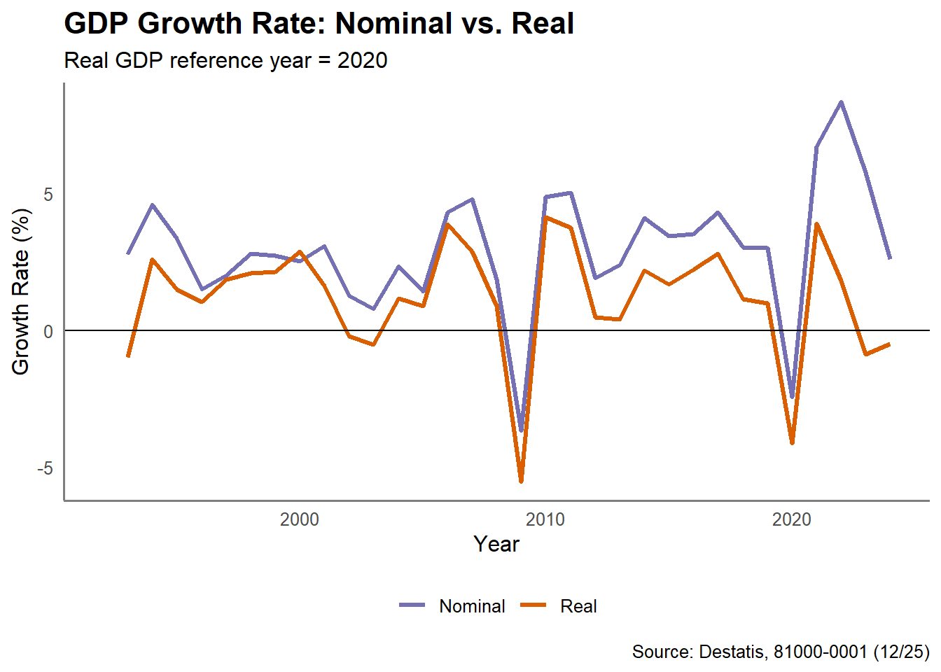

Industry

Gross Value Added by Sector

industry_raw <- gen_table("81000-0013", database = "genesis")

industry <- industry_raw |>
  filter(value_unit == "unit app.",
         `2_variable_attribute_label`== "Price-adjusted, chain-linked volume data (bn EUR)") |>   
  mutate(
    time = as.integer(time),
    value = as.numeric(value)
  ) |>
  select(time, `3_variable_attribute_label`, value) |>
  rename(sector = `3_variable_attribute_label`,
         gva_real = value)|>
  setDT() 

#industry_selected <- industry |>
  #filter(sector %in% sectors_selected)

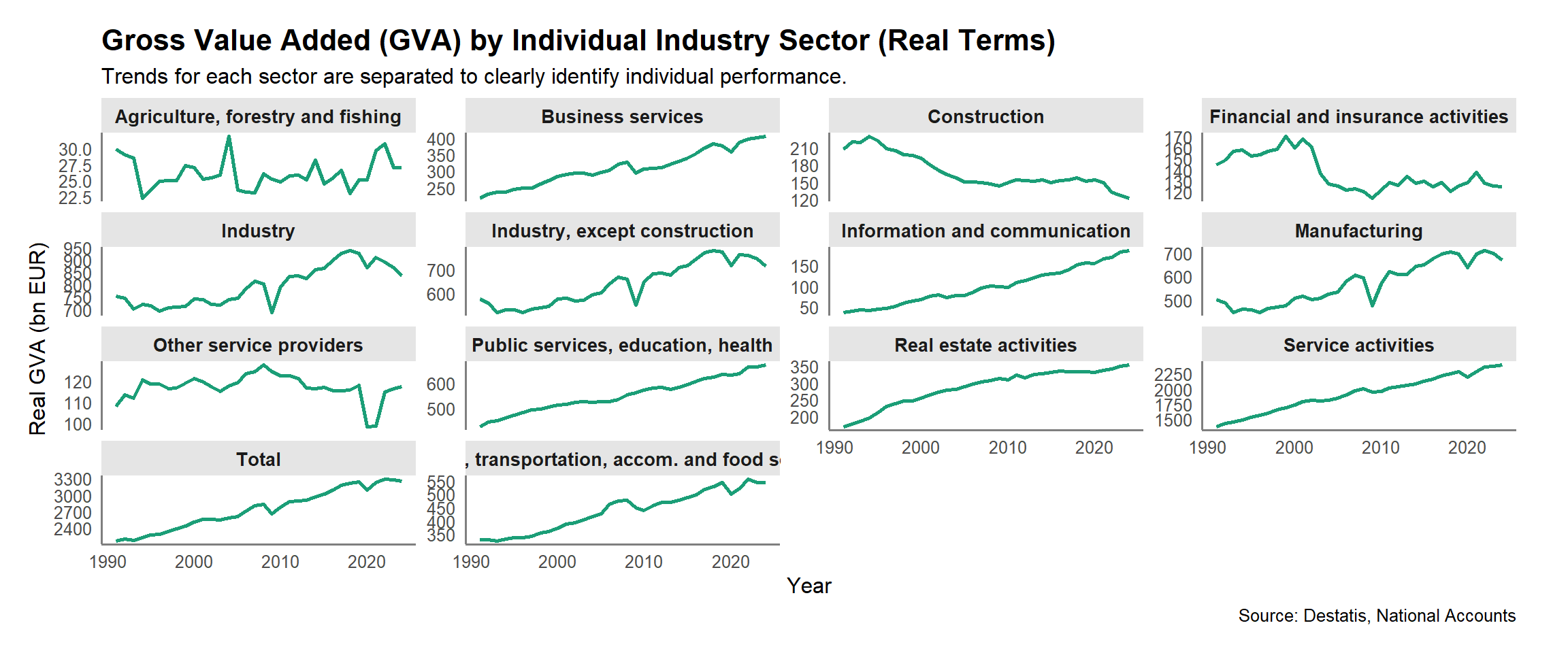
ggplot(industry, aes(x = time, y = gva_real)) +
  geom_line(color = colors["Accent"], linewidth = 1.0) +
  facet_wrap(~ sector, scales = "free_y", strip.position = "top") +
  scale_color_discrete() +
  labs(
    title = "Gross Value Added (GVA) by Individual Industry Sector (Real Terms)",
    subtitle = "Trends for each sector are separated to clearly identify individual performance.",
    x = "Year",
    y = "Real GVA (bn EUR)",
    caption = "Source: Destatis, National Accounts"
  ) +
  theme_set() + 
  theme(
    plot.margin = unit(c(5.5, 10, 5.5, 5.5), "mm"), 
    strip.background = element_rect(fill = "grey90", color = NA),
    strip.text = element_text(face = "bold", size = 10),
    legend.position = "none"
  )

industry_filtered <- industry |>
  filter(time >= 2018) |>
  filter(!grepl("Total|Gesamt|Summe|wirtschaft gesamt", sector, ignore.case = TRUE))

index_base <- industry_filtered |>
  filter(time == 2018) |>
  select(sector, gva_real) |>
  rename(size_metric = gva_real) 

industry_indexed_sized <- industry_filtered |>
  left_join(index_base, by = "sector") |>
  mutate(
    gva_index = (gva_real / size_metric) * 100
  ) |>
  select(time, sector, gva_index, size_metric)

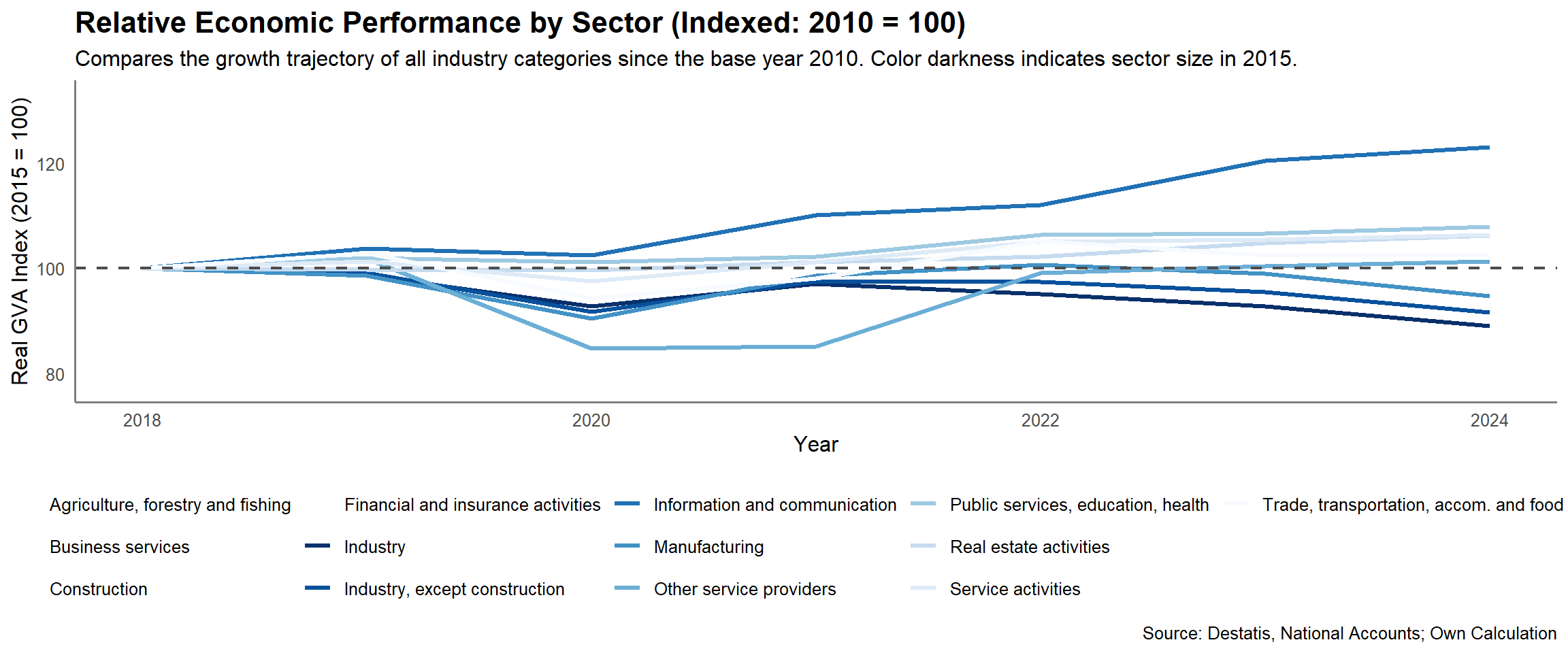
ggplot(industry_indexed_sized, aes(x = time, y = gva_index, group = sector, color = sector)) +
  geom_line(linewidth = 1.2) +
  geom_hline(yintercept = 100, linetype = "dashed", color = "grey30", linewidth = 0.8) +
  labs(
    title = "Relative Economic Performance by Sector (Indexed: 2010 = 100)",
    subtitle = "Compares the growth trajectory of all industry categories since the base year 2010. Color darkness indicates sector size in 2015.",
    x = "Year",
    y = "Real GVA Index (2015 = 100)",
    color = "GVA 2010 (bn EUR)",
    caption = "Source: Destatis, National Accounts; Own Calculation"
  ) +
  scale_color_brewer(palette = "Blues", direction = -1) +
  # Map continuous size metric (numeric) to a sequential blue gradient
  #scale_color_gradient(low = "#C6DBEF", high = "#08519C") +
  theme_set()